11 Creating map Visualizations with {ggplot2}
In addition to the classic graphics presented in Chapter 5, there is a whole range of extensions available in {ggplot2}.
For maps and spatial data work, the {sf} package is available and allows to plot “Choropleths” (thematic maps) with {ggplot2}. The great thing is: we can process {sf} data with the familiar {tidyverse} commands. To create a map, we need a shapefile that contains information about the areas to be displayed. For Germany, the Geodata Center of the Federal Agency for Cartography and Geodesy provides shapefiles for municipalities, districts, and states.
Here you can find shapefiles for different years.
Usually, the results or data we want to display are based on a specific area status (due to territorial reforms, there are continuous changes in both areas and identifiers). To avoid complex record linkage, it is helpful to use the shapefile for the relevant year. On this page you can also find past territorial statuses. The files with the name scheme vg250_01-01.utm32s.shape.ebenen.zip contain the necessary information that we will use in the following.
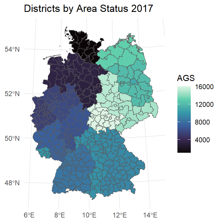
We can then join these shapefiles with data based on the AGS (Official Municipality Key) and display them as a map:
To load a shapefile, we first install {sf} and then load it with library(). The actual loading is done by the read_sf() command, where we need to specify both the file path in the unpacked folder with the shapefiles and the layer, i.e., the level. In the BKG shapefiles, there are the following layers:
VG250_LAN: Federal States (2-digit AGS)VG250_KRS: Districts and Independent Cities (5-digit AGS)VG250_GEM: Cities and Municipalities (8-digit AGS)
So, if we want to load the federal states, we proceed as follows:
lan17 <- sf::read_sf("./orig/vg250_2017.utm32s.shape.ebenen/vg250_ebenen",
                     layer="VG250_LAN")
The lan17 object can now be used for a ggplot() command. lan17 also contains the sea areas, which we can filter to land areas only using a filter() command (GF = 4):
ggplot(lan17) +
geom_sf(size = .1) +
labs(title = "Federal States by Area Status 2017") +
theme_void()
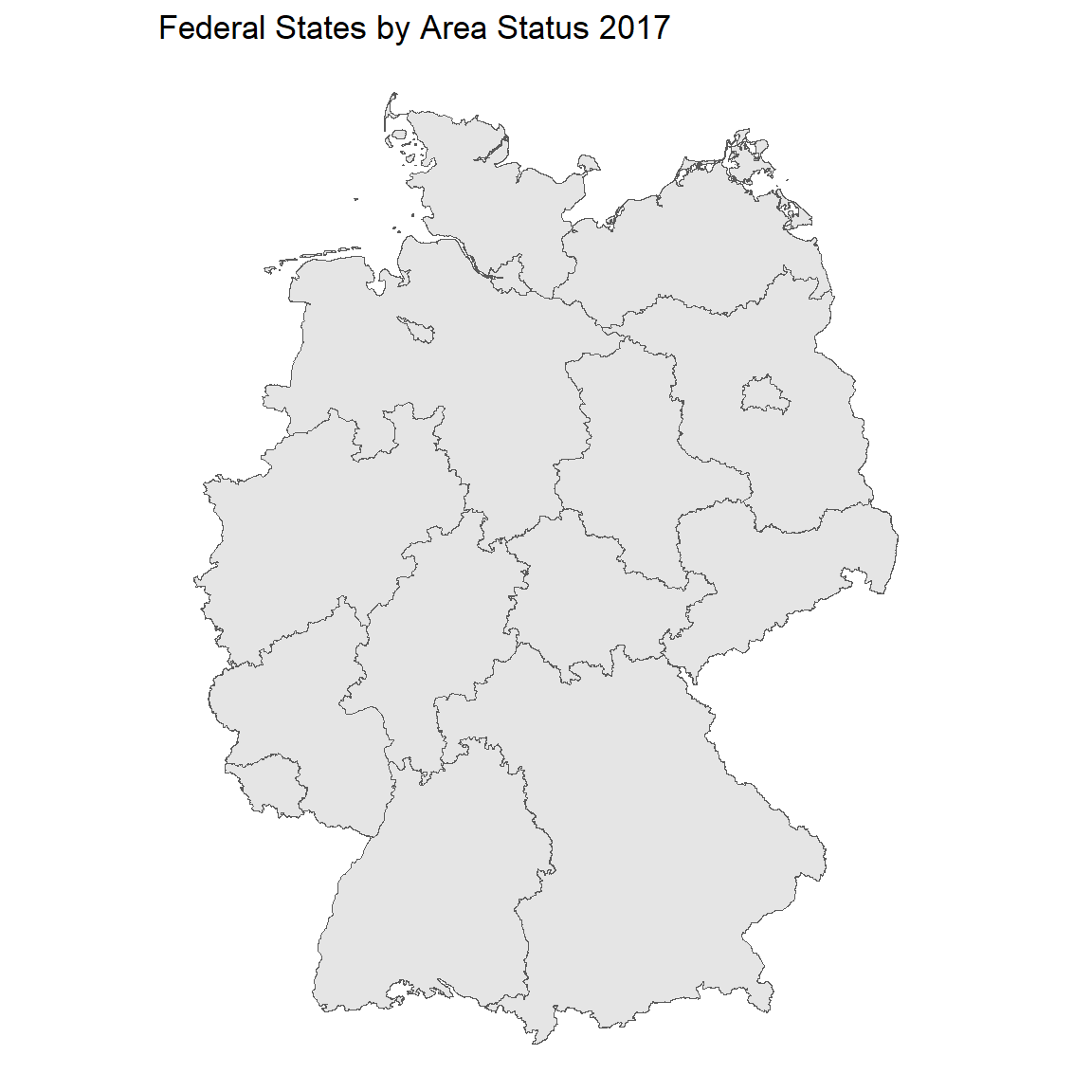
ggplot(lan17 %>% filter(GF==4)) +
geom_sf(size = .1) +
labs(title = "Federal States by Area Status 2017") +
theme_void()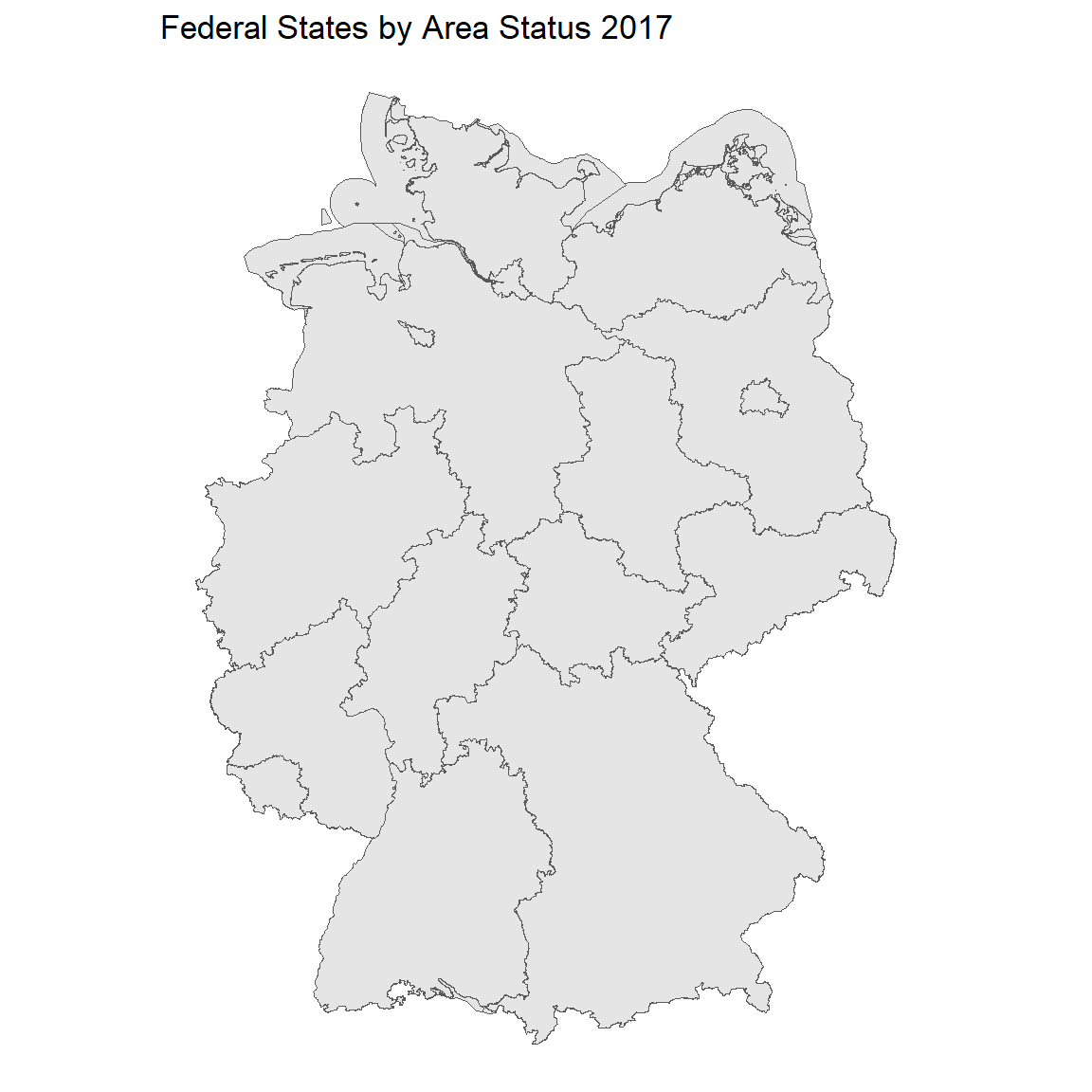
If we now want to color the federal states, for example, by the unemployment rate, we need to incorporate this data. For simplicity, I will simulate the values here:
alo_df <-
  data.frame(ags = unique(lan17$AGS),
             alq = sample(seq(.03,.095,.001) ,size = 16,replace = T))
head(alo_df)
ags alq
1 01 0.052
2 02 0.033
3 03 0.094
4 04 0.060
5 05 0.032
6 06 0.071We can now join the alo_df data to the lan17 shapefile using a left_join().
lan17 %>% filter(GF==4) %>% left_join(alo_df,by = join_by("AGS"=="ags"))lan17 %>% filter(GF==4) %>% left_join(alo_df,by = join_by("AGS"=="ags")) %>%
select(AGS,GEN,alq) %>%
head()Simple feature collection with 6 features and 3 fields
Geometry type: MULTIPOLYGON
Dimension: XY
Bounding box: xmin: 280371.1 ymin: 5471366 xmax: 674202.3 ymax: 6101444
Projected CRS: ETRS89 / UTM zone 32N
# A tibble: 6 × 4
AGS GEN alq geometry
<chr> <chr> <dbl> <MULTIPOLYGON [m]>
1 01 Schleswig-Holstein 0.052 (((464810.7 6100447, 464936.7 6100389, 465073…
2 02 Hamburg 0.033 (((578219 5954278, 578433.9 5954189, 578557.7…
3 03 Niedersachsen 0.094 (((479451.1 5971302, 479365.8 5971220, 479213…
4 04 Bremen 0.06 (((466930.3 5897851, 467015.7 5897733, 467379…
5 05 Nordrhein-Westfalen 0.032 (((477607.3 5818769, 477708 5818638, 477758.9…
6 06 Hessen 0.071 (((534242 5721822, 534214.5 5721748, 534149.4…The syntax for the actual plot is then similar to any other ggplot() - with fill = we can specify a fill color and with scale_fill_... we can choose a color palette:
library(scico)
lan17 %>%
  filter(GF==4) %>%
  left_join(alo_df,by = join_by("AGS"=="ags")) %>%
  ggplot() +
      geom_sf(size = .1, aes(fill = alq))  +
      labs(title = "Unemployment Rate for Federal States",
           subtitle = "(not real data)",
           fill = "Unemployment\nrate") +
      scale_fill_scico(palette = "oslo") + # requires scico package
      theme_void()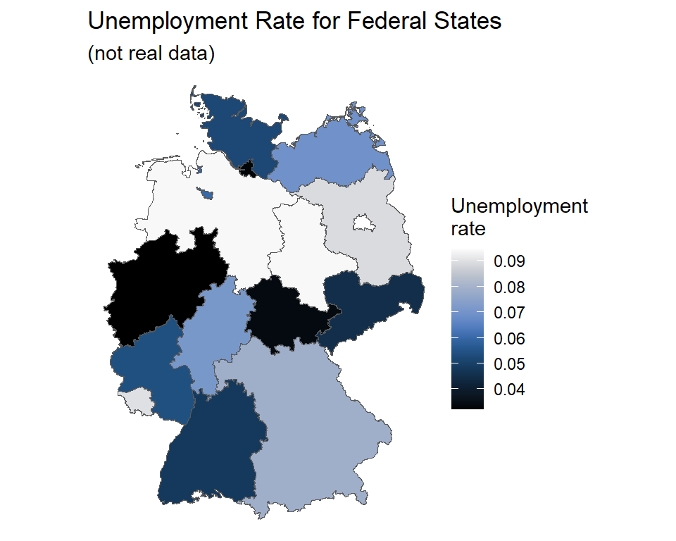
11.1 Modify sf shape data.frames
We can use the familiar {dplyr} functions to amend the sf data. Here’s are rather silly example how to combine Saxony, Saxony-Anhalt and Thuringa into one unit:
lan17_15länder <-
  lan17 %>%
  filter(GF==4) %>%
  mutate(newid = case_when(as.numeric(AGS)>13 ~ "17",  TRUE ~ AGS)) %>% # same ID for SN, SA, TH
  summarise(geometry = st_union(geometry),.by = newid) # summarise -> combine based on newid

ggplot(lan17_15länder) +
  geom_sf(size = .1, aes(fill = as.numeric(newid)) )  +
  scale_fill_scico(palette = "oslo") + # requires scico package
  theme_minimal()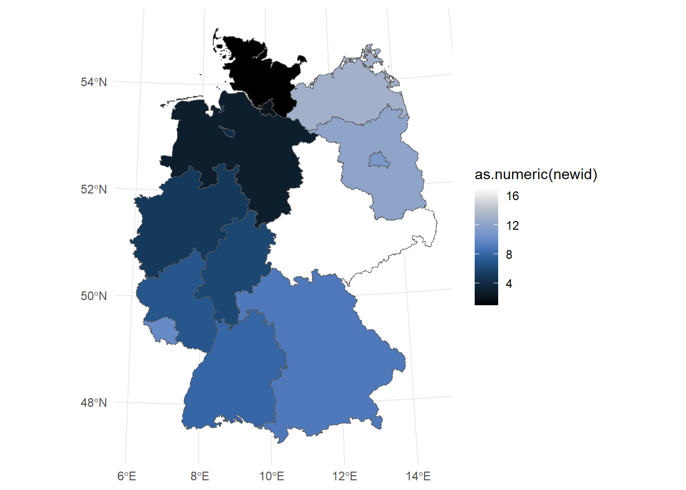
11.2 Exercise
Create a map yourself - for the country, district, or municipality level.
- You can find the shapefile for the year 2017 in the course folder under
/origin the Quickablage.