7  Regression Models: Extensions

After covering the basics of regression models, this chapter explores some useful extensions of regression models in R.

library(tidyverse)

dat1 <- data.frame(id = 1:8,
                   var1 = c(2,1,2,5,7,8,9,5),
                   var2 = c(2,2,1,9,7,4,25,3),
                   educ = c(3,1,2,2,1,3,2,-1),
                   gend = c(2,1,1,2,1,2,1,2),
                   x = c(2,1,2,4,1,NA,NA,NA))
dat1$ed_fct <- factor(dat1$educ, levels = 1:3,
                        labels = c("basic","medium","high"))
dat1
  id var1 var2 educ gend  x ed_fct
1  1    2    2    3    2  2   high
2  2    1    2    1    1  1  basic
3  3    2    1    2    1  2 medium
4  4    5    9    2    2  4 medium
5  5    7    7    1    1  1  basic
6  6    8    4    3    2 NA   high
7  7    9   25    2    1 NA medium
8  8    5    3   -1    2 NA   <NA>

7.1 Keeping Only Complete Rows

When we compare models m1 and m3, we see different sample sizes:

m1 <- lm(var2 ~ var1, data = dat1)  
m4 <- lm(var2 ~ ed_fct + var1, data = dat1)
modelsummary(list("m1"=m1,"m4"=m4), gof_omit = "IC|RM|Log|F")
tinytable_wlxerlegku5cm0jvsolp
m1 m4
(Intercept) -2.340 -2.511
(4.345) (5.681)
var1 1.839 1.753
(0.773) (0.835)
ed_fctmedium 4.830
(6.038)
ed_fcthigh -3.253
(6.554)
Num.Obs. 8 7
R2 0.486 0.700
R2 Adj. 0.400 0.400

It appears that in model m4, one case is lost with ed_fct. Why is that? It’s worth taking a look at the data:

dat1
  id var1 var2 educ gend  x ed_fct
1  1    2    2    3    2  2   high
2  2    1    2    1    1  1  basic
3  3    2    1    2    1  2 medium
4  4    5    9    2    2  4 medium
5  5    7    7    1    1  1  basic
6  6    8    4    3    2 NA   high
7  7    9   25    2    1 NA medium
8  8    5    3   -1    2 NA   <NA>

The value for ed_fct is missing for id = 8.

To compare the models, we should use only the rows where ed_fct values are available. We can manually select these rows (excluding id=8), but this can be cumbersome with larger datasets.

7.1.1 complete.cases()

Here, complete.cases() is helpful. This function creates a logical variable that is TRUE for all complete cases (i.e., without NA). Incomplete cases are marked as FALSE. We specify which variables to consider for this check and add the variable to the dataset as a new column. For model 1, a case is considered complete if both var2 and var1 are present. So, we select the relevant variables with select() and apply complete.cases to this selection:

dat1 %>% select(var1, var2) %>% complete.cases(.) 
[1] TRUE TRUE TRUE TRUE TRUE TRUE TRUE TRUE
dat1$compl_m1 <- dat1 %>% select(var1, var2) %>% complete.cases(.) 
dat1
  id var1 var2 educ gend  x ed_fct compl_m1
1  1    2    2    3    2  2   high     TRUE
2  2    1    2    1    1  1  basic     TRUE
3  3    2    1    2    1  2 medium     TRUE
4  4    5    9    2    2  4 medium     TRUE
5  5    7    7    1    1  1  basic     TRUE
6  6    8    4    3    2 NA   high     TRUE
7  7    9   25    2    1 NA medium     TRUE
8  8    5    3   -1    2 NA   <NA>     TRUE

Note: if we do not specify variables, NA will be considered from all variables, including x, which we are not interested in here:

dat1 %>% complete.cases(.) 
[1]  TRUE  TRUE  TRUE  TRUE  TRUE FALSE FALSE FALSE
dat1$compl <- dat1 %>% complete.cases(.) 
dat1
  id var1 var2 educ gend  x ed_fct compl_m1 compl
1  1    2    2    3    2  2   high     TRUE  TRUE
2  2    1    2    1    1  1  basic     TRUE  TRUE
3  3    2    1    2    1  2 medium     TRUE  TRUE
4  4    5    9    2    2  4 medium     TRUE  TRUE
5  5    7    7    1    1  1  basic     TRUE  TRUE
6  6    8    4    3    2 NA   high     TRUE FALSE
7  7    9   25    2    1 NA medium     TRUE FALSE
8  8    5    3   -1    2 NA   <NA>     TRUE FALSE

We do the same for model m4, which includes ed_fct in addition to var2 and var1:

dat1$compl_m4 <- dat1 %>% select(var1, var2, ed_fct) %>% complete.cases(.)

Here’s how it looks in the dataset:

dat1
  id var1 var2 educ gend  x ed_fct compl_m1 compl_m4
1  1    2    2    3    2  2   high     TRUE     TRUE
2  2    1    2    1    1  1  basic     TRUE     TRUE
3  3    2    1    2    1  2 medium     TRUE     TRUE
4  4    5    9    2    2  4 medium     TRUE     TRUE
5  5    7    7    1    1  1  basic     TRUE     TRUE
6  6    8    4    3    2 NA   high     TRUE     TRUE
7  7    9   25    2    1 NA medium     TRUE     TRUE
8  8    5    3   -1    2 NA   <NA>     TRUE    FALSE

7.1.2 Finding Cases with Missing Values

Now, we can filter by these variables and examine these cases more closely. We filter for cases that are included in m1 (i.e., compl_m1 = TRUE) but not in m4 (compl_m4 = FALSE):

dat1 %>% filter(compl_m1 == T & compl_m4 == F) 
  id var1 var2 educ gend  x ed_fct compl_m1 compl_m4
1  8    5    3   -1    2 NA   <NA>     TRUE    FALSE

7.1.3 Calculating Models with Only Complete Cases

We can now create model m1 to include only cases that are also considered in model m4:

m1_m4vars <- lm(var2 ~ var1, data = filter(dat1, compl_m4 == T))
modelsummary(list("m1"=m1,"m1 with m4vars"=m1_m4vars,"m4"=m4), gof_omit = "IC|RM|Log|F")
tinytable_rc35evn7tax8cahz4sg8
m1 m1 with m4vars m4
(Intercept) -2.340 -1.832 -2.511
(4.345) (4.646) (5.681)
var1 1.839 1.848 1.753
(0.773) (0.814) (0.835)
ed_fctmedium 4.830
(6.038)
ed_fcthigh -3.253
(6.554)
Num.Obs. 8 7 7
R2 0.486 0.508 0.700
R2 Adj. 0.400 0.409 0.400

Now, both m1 with m4vars and m4 have the same number of cases, allowing for a direct comparison of the results.
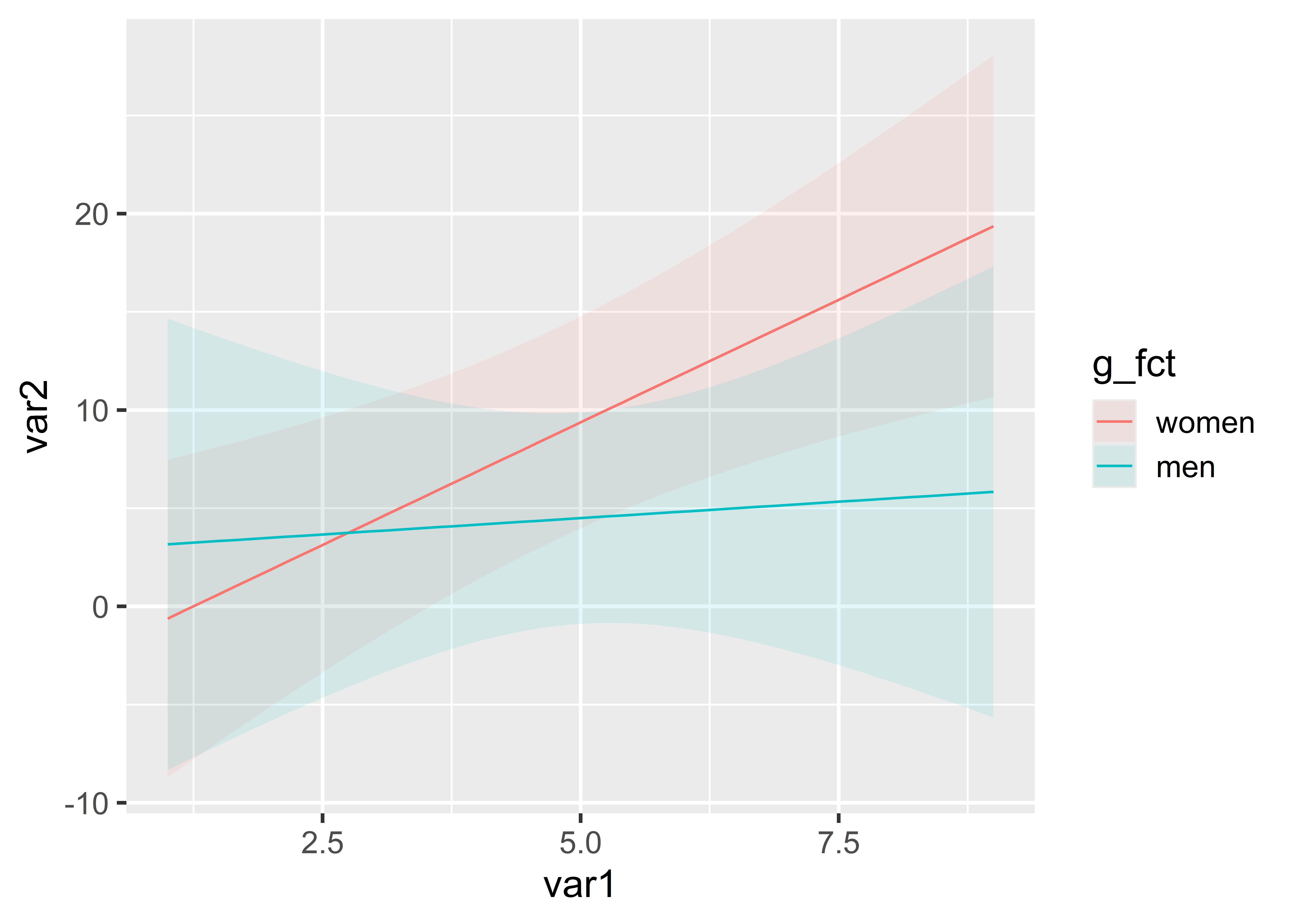
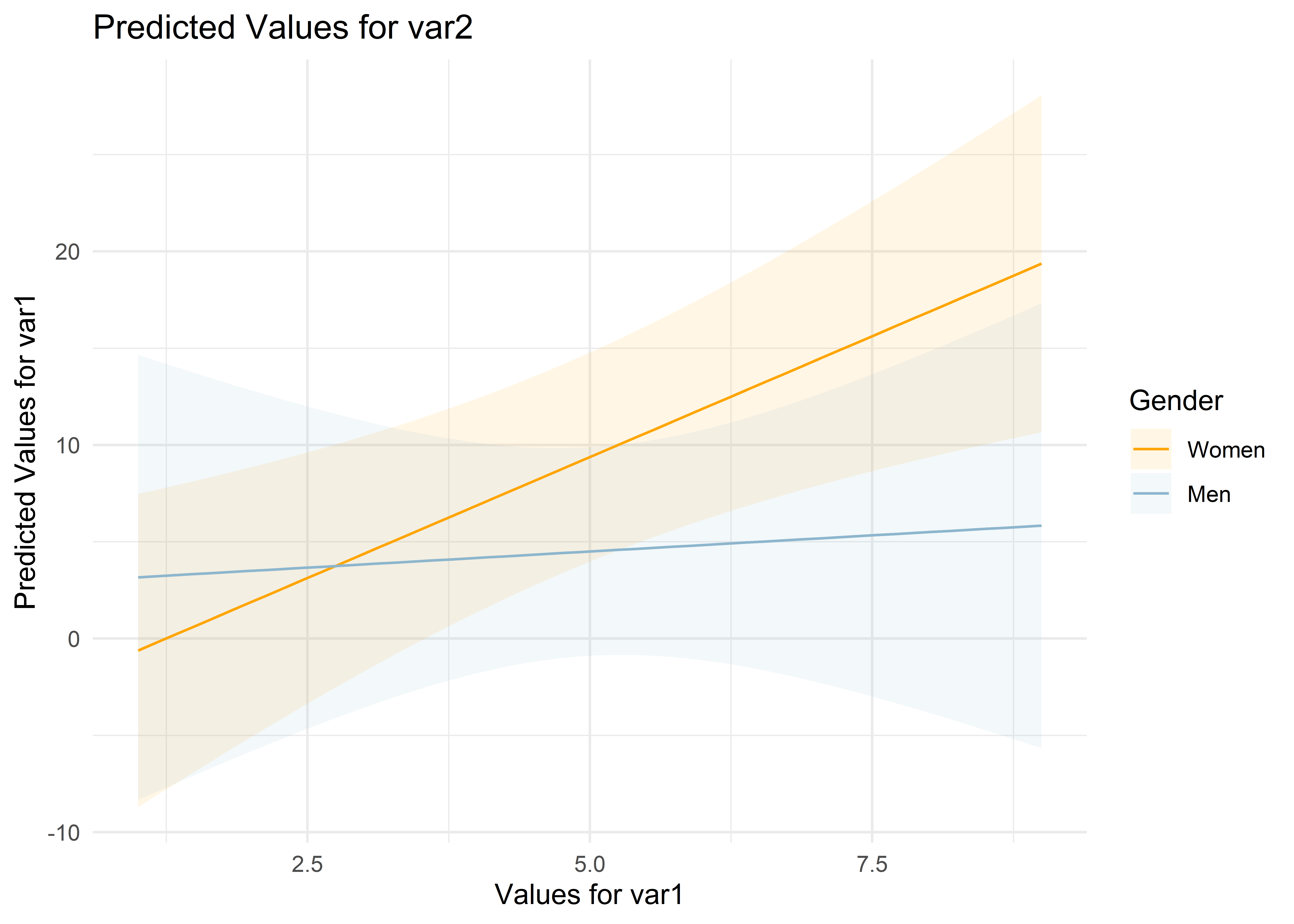
7.2 Interactions

Interactions between two variables can be calculated using *:

dat1$g_fct <- factor(dat1$gend, levels = 1:2,
                     labels = c("women","men"))
m5 <- lm(var2 ~ var1 * g_fct, data = dat1)
summary(m5)

Call:
lm(formula = var2 ~ var1 * g_fct, data = dat1)

Residuals:
      1       2       3       4       5       6       7       8 
-1.5000  2.6145 -0.8827  4.5000 -7.3687 -1.5000  5.6369 -1.5000 

Coefficients:
              Estimate Std. Error t value Pr(>|t|)  
(Intercept)    -3.1117     4.7702  -0.652   0.5498  
var1            2.4972     0.8211   3.041   0.0384 *
g_fctmen        5.9451     8.4973   0.700   0.5227  
var1:g_fctmen  -2.1639     1.5331  -1.411   0.2310  
---
Signif. codes:  0 '***' 0.001 '**' 0.01 '*' 0.05 '.' 0.1 ' ' 1

Residual standard error: 5.493 on 4 degrees of freedom
Multiple R-squared:  0.7244,    Adjusted R-squared:  0.5177 
F-statistic: 3.504 on 3 and 4 DF,  p-value: 0.1286

avg_slopes() from {marginaleffects} helps to calculate the marginal effects/slopes of a one-unit increase in var1 for each subgroup of g_fct:

avg_slopes(m5,
           variables = "var1",
           by = "g_fct")

 g_fct Estimate Std. Error     z Pr(>|z|)   S  2.5 % 97.5 %
 women    2.497      0.821 3.041  0.00236 8.7  0.888   4.11
 men      0.333      1.295 0.257  0.79684 0.3 -2.204   2.87

Term: var1
Type:  response 
Comparison: mean(dY/dX)
Columns: term, contrast, g_fct, estimate, std.error, statistic, p.value, s.value, conf.low, conf.high, predicted_lo, predicted_hi, predicted 

Interactions should always be visualized. plot_predictions() from {marginaleffects} is a very helpful function to plot the predicted values :

plot_predictions(m5, condition = c("var1", "g_fct"))

We can modify this plot using familiar {ggplot2} commands:

plot_predictions(m5, condition = c("var1", "g_fct")) + 
  scale_color_manual(values = c("orange","lightskyblue3"), breaks = c("women","men"), labels=c("Women","Men")) +
  scale_fill_manual(values = c("orange","lightskyblue3"), breaks = c("women","men"), labels=c("Women","Men")) +
  labs(title = "Predicted Values for var2",
       color = "Gender", fill = "Gender",
       x = "Values for var1",
       y = "Predicted Values for var1") +
  theme_minimal()

Alternatively, we can create the “marginsplot” step by step ourselves

7.3 Quadratic Terms & Polynomials

m6 <- lm(var2 ~ var1 + I(var1^2), data = dat1 %>% filter(id != 7))
summary(m6)

Call:
lm(formula = var2 ~ var1 + I(var1^2), data = dat1 %>% filter(id != 
    7))

Residuals:
      1       2       3       4       5       6       7 
-0.5443  1.4334 -1.5443  3.2043  1.2713 -1.0248 -2.7957 

Coefficients:
            Estimate Std. Error t value Pr(>|t|)
(Intercept)  -1.8580     3.4066  -0.545    0.614
var1          2.6481     1.9083   1.388    0.238
I(var1^2)    -0.2235     0.2110  -1.059    0.349

Residual standard error: 2.524 on 4 degrees of freedom
Multiple R-squared:  0.5099,    Adjusted R-squared:  0.2648 
F-statistic: 2.081 on 2 and 4 DF,  p-value: 0.2402

Again, {marginaleffects} provides a helpful function to visualize the shape of predicted values:

plot_predictions(m6, condition = "var1") # conditional adjusted predictions 

plot_slopes(m6, variables = "var1", condition = "var1") # conditional marginal effects

7.4 Logistic regression model

For binary dependent variables, logistic regression models are a widely used tool. We can fit logistic regression models in R using glm() - for an example, we turn to PSM0100 (Usage of social networks yes = 1, no = 2) :

\[\begin{equation*} \widehat{Logit(soc\_med=1)} = \widehat{ln\left(\frac{P(soc\_med=1)}{1-P(soc\_med=1)}\right)} = \hat\beta0 + \hat{\beta1}\times \texttt{palter} \end{equation*}\]

pend10 <- haven::read_dta("./orig/PENDDAT_cf_W13.dta",
                          col_select = c("palter","PSM0100")) %>% 
  filter(PSM0100>0) %>% 
  mutate(soc_med = 2- PSM0100)  # convert into 0/1 dummy variable

pend10 %>% count(soc_med,PSM0100) # check: soc_med = 1 -> yes, soc_med = 0 -> no
# A tibble: 2 × 3
  soc_med PSM0100       n
    <dbl> <dbl+lbl> <int>
1       0 2 [No]     2873
2       1 1 [Yes]    2589
m2 <- glm(soc_med ~ palter, family = "binomial", data = pend10)
summary(m2)

Call:
glm(formula = soc_med ~ palter, family = "binomial", data = pend10)

Coefficients:
             Estimate Std. Error z value Pr(>|z|)    
(Intercept)  3.194321   0.107660   29.67   <2e-16 ***
palter      -0.073518   0.002315  -31.75   <2e-16 ***
---
Signif. codes:  0 '***' 0.001 '**' 0.01 '*' 0.05 '.' 0.1 ' ' 1

(Dispersion parameter for binomial family taken to be 1)

    Null deviance: 7557.2  on 5461  degrees of freedom
Residual deviance: 6217.5  on 5460  degrees of freedom
AIC: 6221.5

Number of Fisher Scoring iterations: 3

The interpretation of the \(\beta\) coefficients from a logistic regression model pertains to the logits (the logarithms of the odds): There is a statistically significant relationship at the 0.001 level between age and the probability of using social media. With each additional year of age, there is a decrease of 0.073518 in the logits* of the respondents using social media.*

7.4.1 average marginal effects

Logits are quite cumbersome—so how does the probability of \(\texttt{soc\_med} = 1\) change with palter? Here, we face the challenge that the derivative of the “inverse function” is not as straightforward as in the case of OLS. If we modify the regression equation from above1 with exp() and \(p=\frac{Odds}{1+Odds}\), we get:

\[\begin{equation*} \widehat{P(soc\_med=1)} = \frac{e^{\hat\beta0+\hat\beta1 \times \texttt{palter}}}{1+e^{\hat\beta0+\hat{\beta1}\times \texttt{palter}}} \end{equation*}\]

We would need to differentiate this expression with respect to palter to determine how the predicted probability of \(\texttt{soc\_med} = 1\) changes with each additional year of respondent age. Given that palter appears in both the exponent of the e function and both the numerator and denominator (“top and bottom”), the differentiation becomes significantly more complex than in the previous lm() models.

For our purposes, it is crucial to note that to compute changes in the predicted probabilities, we need the so-called marginal effects from the {marginaleffects} package. This package includes the avg_slopes() function, which allows us to calculate a \(\beta\) representing the change in the probability of \(\texttt{soc\_med} = 1\) in relation to palter. This is known as the average marginal effect, as it provides the average marginal change in the dependent variable for a one-unit increase in the independent variable.

fdz_install("marginaleffects") # nur einmal nötig
library(marginaleffects)
avg_slopes(m2)

 Estimate Std. Error     z Pr(>|z|)   S   2.5 %  97.5 %
  -0.0142   0.000266 -53.4   <0.001 Inf -0.0147 -0.0137

Term: palter
Type:  response 
Comparison: mean(dY/dX)
Columns: term, contrast, estimate, std.error, statistic, p.value, s.value, conf.low, conf.high, predicted_lo, predicted_hi, predicted 

With each additional year of age, there is on average a decrease of 0.01419 (1.419 percentage points) in the probability of using social media.

7.5 Weighted Regression Model

The {survey} package allows including weights when fitting regression model:

fdz_install("survey")
library(survey)
pend <- haven::read_dta("./orig/PENDDAT_cf_W13.dta") %>% filter(netges > 0 , palter > 0, azges1 > 0) %>% 
  mutate(zpsex_fct = factor(zpsex, levels = 1:2, labels = c("M","W")))
wgt_df <- haven::read_dta("./orig/pweights_cf_W13.dta")
pend_wgt <- pend %>% left_join(wgt_df, by = join_by(pnr,welle))

modx <- lm(netges ~ palter + I(palter^2),data=pend) # conventional lm() model

# create new data.frame including weights using svydesign() from survey-package
pend_weighted <- svydesign(id      = ~pnr, # id variable
                           weights = ~wqp, # weight variable
                           data    = pend_wgt) # original unweighted data 

# family = gaussian() provides a linear regression model, like lm() - but respecting weights
survey_modx <- svyglm(netges ~ palter + I(palter^2), 
                    family = gaussian(), data = etb18,design = pend_weighted)

modelsummary(list("lm()"=modx,"svyglm()"= survey_modx),gof_omit = "RM|IC|Log")
tinytable_fu7vjx5bc5ehko34nu0r
lm() svyglm()
(Intercept) 811.753 463.721
(354.363) (504.015)
palter 24.640 53.580
(17.071) (26.471)
I(palter^2) -0.147 -0.489
(0.197) (0.314)
Num.Obs. 7996 7996
R2 0.004 0.007
R2 Adj. 0.004 -2.252
F 15.525 8.495

7.6 “Robust” Standard Errors

Often, standard errors need to be adjusted for violations of general assumptions (homoscedasticity, etc.).

The good news is that R offers several ways to correct standard errors, including with {sandwich} or {estimatr}.

A very simple option is the correction of standard errors in {modelsummary}, which we will look at in more detail:

We can request heteroskedasticity-consistent (HC) “robust” standard errors with the vcov option HC in modelsummary(). The help page for {modelsummary} provides a list of all options.

One option is also stata, to replicate results from Stata’s , robust. More here about the background and differences.

We can estimate the following model:

mod1 <- lm(netges ~ palter + I(palter^2),data=pend)

In the modelsummary(), we can now display the same model with different adjustments for the standard errors:

library(modelsummary)
modelsummary(list(mod1,mod1,mod1,mod1),vcov = c("classical","HC","HC2","stata"),gof_omit = "RM|IC|Log")
tinytable_273y6n2y7ak2i7vqq2el
(1) (2) (3) (4)
(Intercept) 811.753 811.753 811.753 811.753
(354.363) (171.599) (171.543) (171.520)
palter 24.640 24.640 24.640 24.640
(17.071) (8.923) (8.920) (8.919)
I(palter^2) -0.147 -0.147 -0.147 -0.147
(0.197) (0.112) (0.112) (0.112)
Num.Obs. 7996 7996 7996 7996
R2 0.004 0.004 0.004 0.004
R2 Adj. 0.004 0.004 0.004 0.004
F 15.525 23.449 23.441 23.440
Std.Errors IID HC HC2 HC1

For clustered SEs, we specify ~clustervariable:

modelsummary(mod1, vcov = c("classical",~pnr), stars = T,gof_omit = "RM|IC|Log|F")
tinytable_f2u3yshx9uzaw7od6jue
(1) (2)
+ p < 0.1, * p < 0.05, ** p < 0.01, *** p < 0.001
(Intercept) 811.753* 811.753**
(354.363) (274.972)
palter 24.640 24.640+
(17.071) (14.475)
I(palter^2) -0.147 -0.147
(0.197) (0.185)
Num.Obs. 7996 7996
R2 0.004 0.004
R2 Adj. 0.004 0.004
Std.Errors IID by: pnr

7.7 Fixed Effects Models with {fixest}

fdz_install("fixest")

{fixest}) offers a wide range of options: logistic FE models, multi-dimensional fixed effects, multiway clustering, etc. And it is very fast, e.g., faster than Stata’s reghdfe. For more details, the vignette is recommended.

The central function for estimating linear FE regression models is feols() - it works very similarly to lm(). We provide a formula following the pattern dependent variable ~ independent variable(s). We simply add the variable that specifies the FEs with |:

library(fixest)
fe_mod1 <- feols(netges ~ palter + I(palter^2) | pnr, data = pend)
fe_mod1
OLS estimation, Dep. Var.: netges
Observations: 7,996
Fixed-effects: pnr: 2,444
Standard-errors: Clustered (pnr) 
              Estimate Std. Error  t value   Pr(>|t|)    
palter      133.811281  14.558248  9.19144  < 2.2e-16 ***
I(palter^2)  -0.848429   0.154417 -5.49441 4.3261e-08 ***
---
Signif. codes:  0 '***' 0.001 '**' 0.01 '*' 0.05 '.' 0.1 ' ' 1
RMSE: 1,222.2     Adj. R2: 0.513287
                Within R2: 0.009765

{fixest} automatically clusters the standard errors along the FE variable (here pnr). If we don’t want that, we can request unclustered SEs with the se option = "standard":

summary(fe_mod1, se = 'standard')
OLS estimation, Dep. Var.: netges
Observations: 7,996
Fixed-effects: pnr: 2,444
Standard-errors: IID 
              Estimate Std. Error  t value   Pr(>|t|)    
palter      133.811281  39.896986  3.35392 0.00080209 ***
I(palter^2)  -0.848429   0.429629 -1.97479 0.04834109 *  
---
Signif. codes:  0 '***' 0.001 '**' 0.01 '*' 0.05 '.' 0.1 ' ' 1
RMSE: 1,222.2     Adj. R2: 0.513287
                Within R2: 0.009765
summary(fe_mod1, cluster = ~pnr)
OLS estimation, Dep. Var.: netges
Observations: 7,996
Fixed-effects: pnr: 2,444
Standard-errors: Clustered (pnr) 
              Estimate Std. Error  t value   Pr(>|t|)    
palter      133.811281  14.558248  9.19144  < 2.2e-16 ***
I(palter^2)  -0.848429   0.154417 -5.49441 4.3261e-08 ***
---
Signif. codes:  0 '***' 0.001 '**' 0.01 '*' 0.05 '.' 0.1 ' ' 1
RMSE: 1,222.2     Adj. R2: 0.513287
                Within R2: 0.009765

{modelsummary} shows the clustered SEs:

modelsummary(fe_mod1,gof_omit = "R|IC|Log|F",stars = T)
tinytable_52l6q69a1l2x8zhhd0i4
(1)
+ p < 0.1, * p < 0.05, ** p < 0.01, *** p < 0.001
palter 133.811***
(14.558)
I(palter^2) -0.848***
(0.154)
Num.Obs. 7996
Std.Errors by: pnr

7.8 Multilevel Models with {lme4}

With lmer(), we can estimate a random intercept model by specifying ( 1 | pnr), which indicates that a separate random intercept should be calculated for each pnr:

library(lme4)
ml_m3 <- lmer(netges ~ palter + I(palter^2) + ( 1 | pnr), data=pend)

modelsummary(list(ml_m3),gof_omit = "R|IC|Log|F")
tinytable_nz8pz063k15zkys3vz7i
(1)
(Intercept) 754.388
(392.459)
palter 18.523
(19.083)
I(palter^2) -0.020
(0.222)
SD (Intercept pnr) 1327.674
SD (Observations) 1414.455
Num.Obs. 7996

More about multilevel models and {lme4} in blog posts by Rense Nieuwenhuis and Tristan Mahr.


  1. \(\widehat{Logit(soc\_med=1)} = \widehat{ln\left(\frac{P(soc\_med=1)}{1-P(soc\_med=1)}\right)} = \hat\beta0 + \hat{\beta1}\times \texttt{palter}\)↩︎